The Fourier Analysis – Part 2

Introduction

In the first part of the “Fourier Analysis” article, we have focused on the properties and usages of the Fourier series. We have seen the power of Fourier series as a tool for both decomposing and constructing general periodic functions in terms of “pure” sines and cosines. The physical world, however, is full of interesting aperiodic or non-periodic functions as well as periodic ones. In course of historical development of the Fourier analysis concept, the original idea was extended to aperiodic signals. An aperiodic function never repeats, then it can technically be considered like a periodic function with an infinite period.

In the case of analysis of non-periodic signals, we can generalize the Fourier Series sum into an integral concept named the Fourier Transform. This is an integral transform in which the time domain signal has to be observed from minus infinity to plus infinity. The Fourier transform can also be considered as a special case of the Laplace transform.

The Fourier transform is a fundamental tool for Spectrum analysis. The best way to understand the true nature of a real-world signal is by examining its spectrum. Spectrum analysis is a very important topic in many scientific and technical fields such as biology, astronomy, geo-sciences, and especially in the field of digital signal processing (DSP).

A Brief Review on Complex Numbers and the Phasor Diagram

The concept of ‘complex numbers’ is out of the scope of this article and we just needed it to achieve the main idea. You could refer to the link attached to get more information:

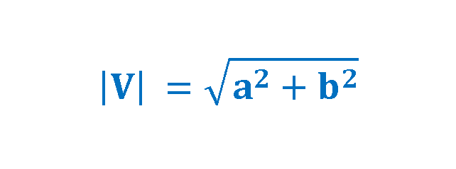
We now define a complex quantity called a “phasor,” which applies to functions that vary sinusoidally with time, like voltages and currents. A phasor is a rotating vector at a constant velocity. Its magnitude corresponds to the amplitude of a signal. It has one end arrowed, to show the direction of action of the quantity. In the vector diagram in Figure 1, the vector of a sinusoidal quantity (V) can be obtained by the vectorial addition of the real (a) and imaginary parts (b), i.e. of the sine and cosine components.

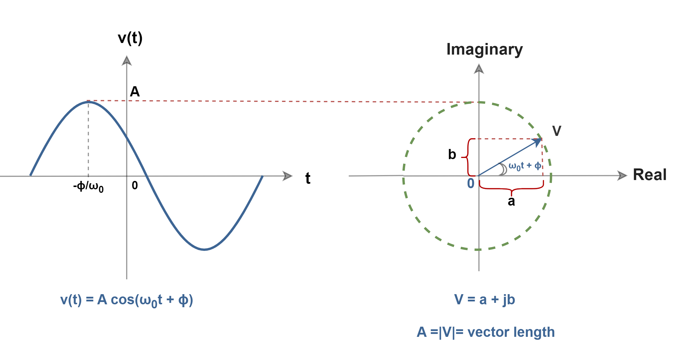
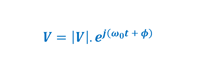
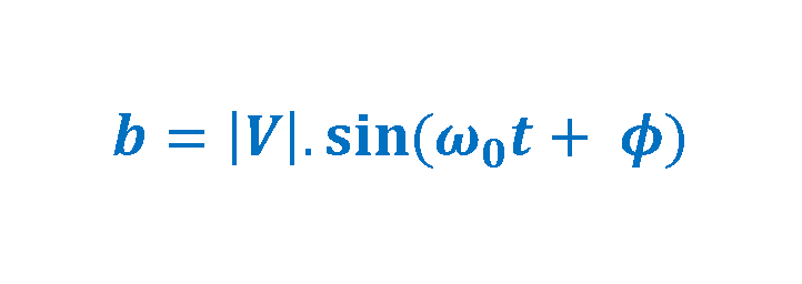
Using Euler’s formula, the polar description of the complex number ‘V’ is given by a magnitude |V| and an argument (ω₀t + ϕ) and satisfies formulas in the set of Equations 1-1 to 1-4:

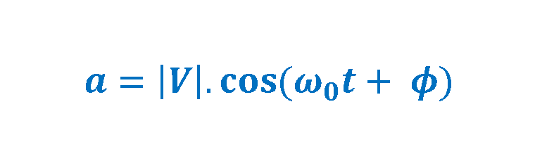
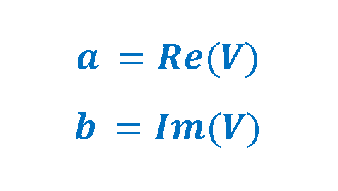
As already mentioned, ‘a’ equals the real part of the complex vector ‘V’ and ‘b’ equals the imaginary part of it. Equation 2 explains these relationships:

The Fourier Transform

The Fourier transform is used similarly to the Fourier series, in that it converts a time-domain function into a frequency-domain representation. However, there are a number of differences:

• Fourier transform can work on aperiodic signals.
• Fourier transform is an infinite sum of infinitesimal sinusoids.
• Non-periodic signals do not have a line spectrum but a continuous spectrum.
• Fourier transform has an inverse transform, that allows for conversion from the frequency domain back to the time domain.

The Fourier transform (or Fourier integral transform) of a function s(t) can be applied by the following integral in Equation 3:

Thus, S(f) represents the frequency domain analysis of the time domain signal s(t) by providing the amplitudes of its frequency components. Equation 3 is also called the forward Fourier transform of the function s(t).

The Inverse Fourier Transform supplies a single real-time-domain signal again from the complex spectrum in the reversed procedure. The inverse transform is given by a similar integral in Equation 4:

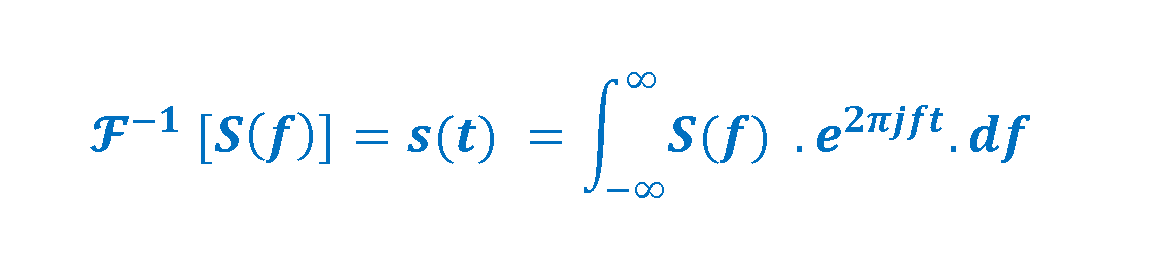
Using these formulas, the aperiodic time-domain signals can be converted to and from the frequency domain, as needed. In the concept of Fourier transforms the pairing metaphor is essential (between equations 3 and 4) so, there is a special notation in many texts to symbolize the bi-directional transforms, as shown in Equation 5:

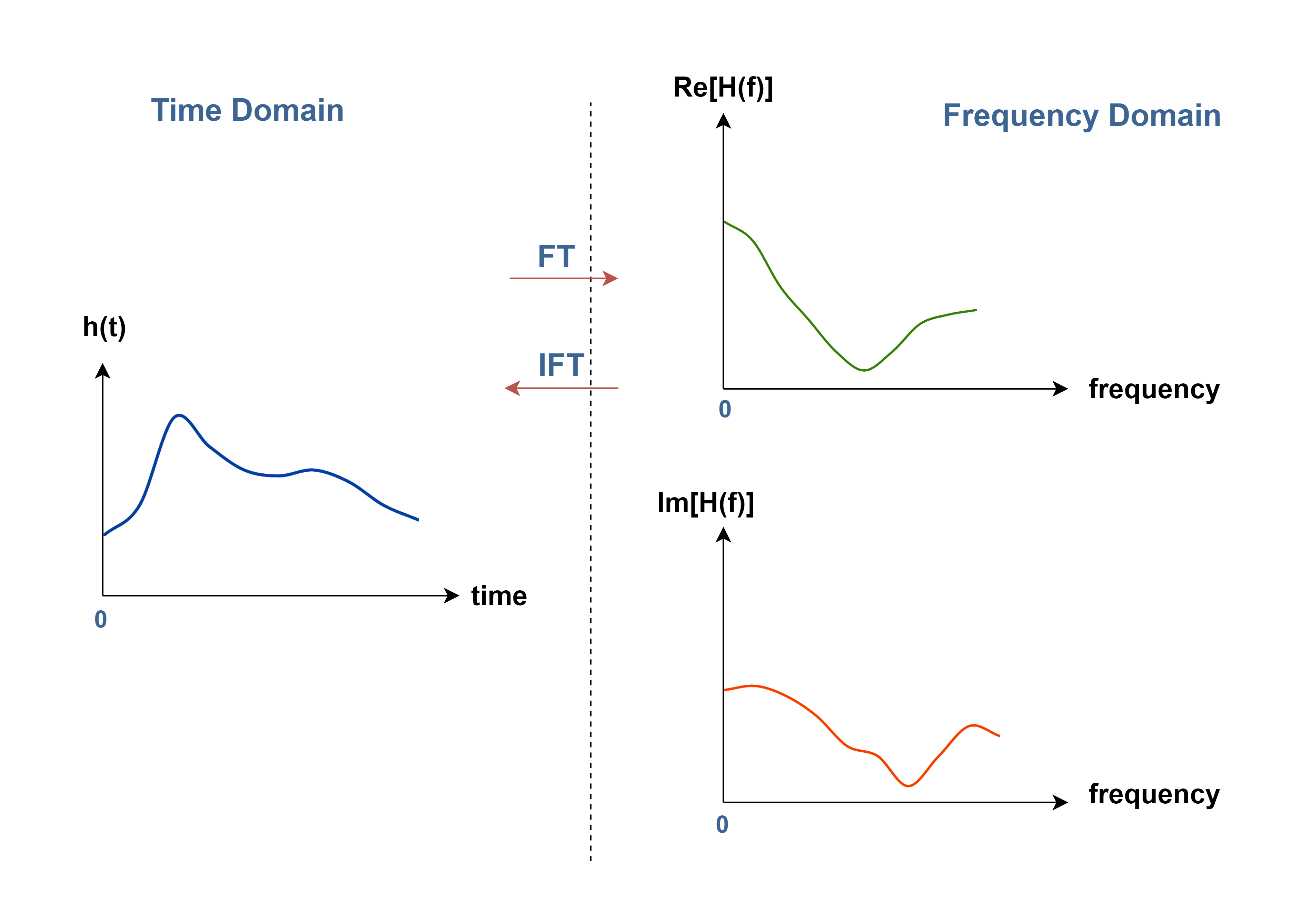
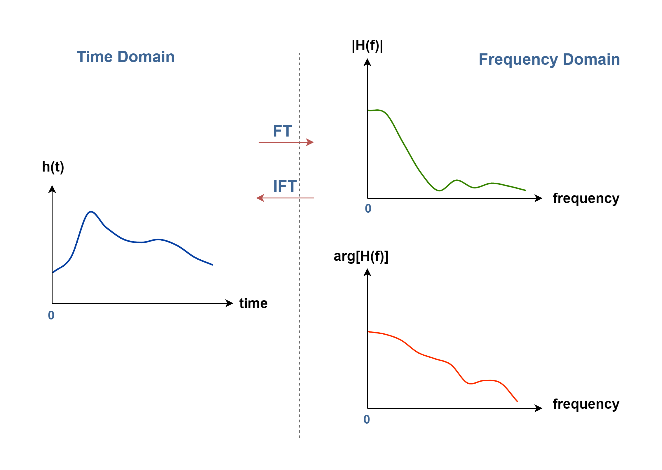
The Fourier transform (FT) alters a real-time-domain signal into a complex spectrum in the frequency domain which is composed of the real-part and the imaginary-part components. The real part accurately describes the amplitude of the cosine component and the imaginary part precisely describes the amplitude of the sine component. Figure 2 explains the transform mechanism graphically for a non-periodic function h(t).

In most of the applications, for each frequency, the magnitude of the vector represents the amplitude of a complex sinusoid with that frequency, and the argument of the complex value represents that complex sinusoid’s phase offset. The graphs of the magnitude and the phase in terms of frequency represent the spectrum of the non-periodic signal. Figure 3 shows the spectrum magnitude |H(f)|and the argument of the function [arg(H)] of an arbitrary signal h(t).

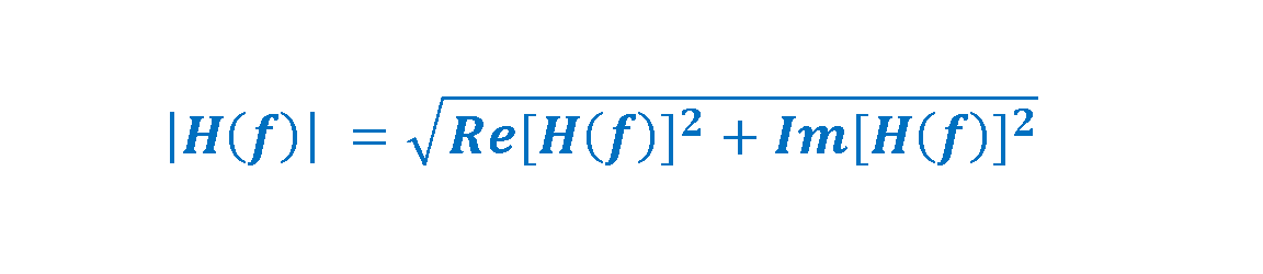
The parameters of the magnitude and the phase (argument) of the transformed vector H(f) are calculated in Equations 6-1 and 6-2.

As already mentioned, when we want to consider the spectrum, in most cases we are mostly looking at the magnitude in terms of frequency rather than phase (or argument).

Examples of Fourier Transforms and Their Graphical Representations

For a better understanding of the mechanism of the Fourier transform, we consider transforms of some specific functions. First, we observe a non-periodic square-shaped function called a single square pulse as shown in Figure 4.

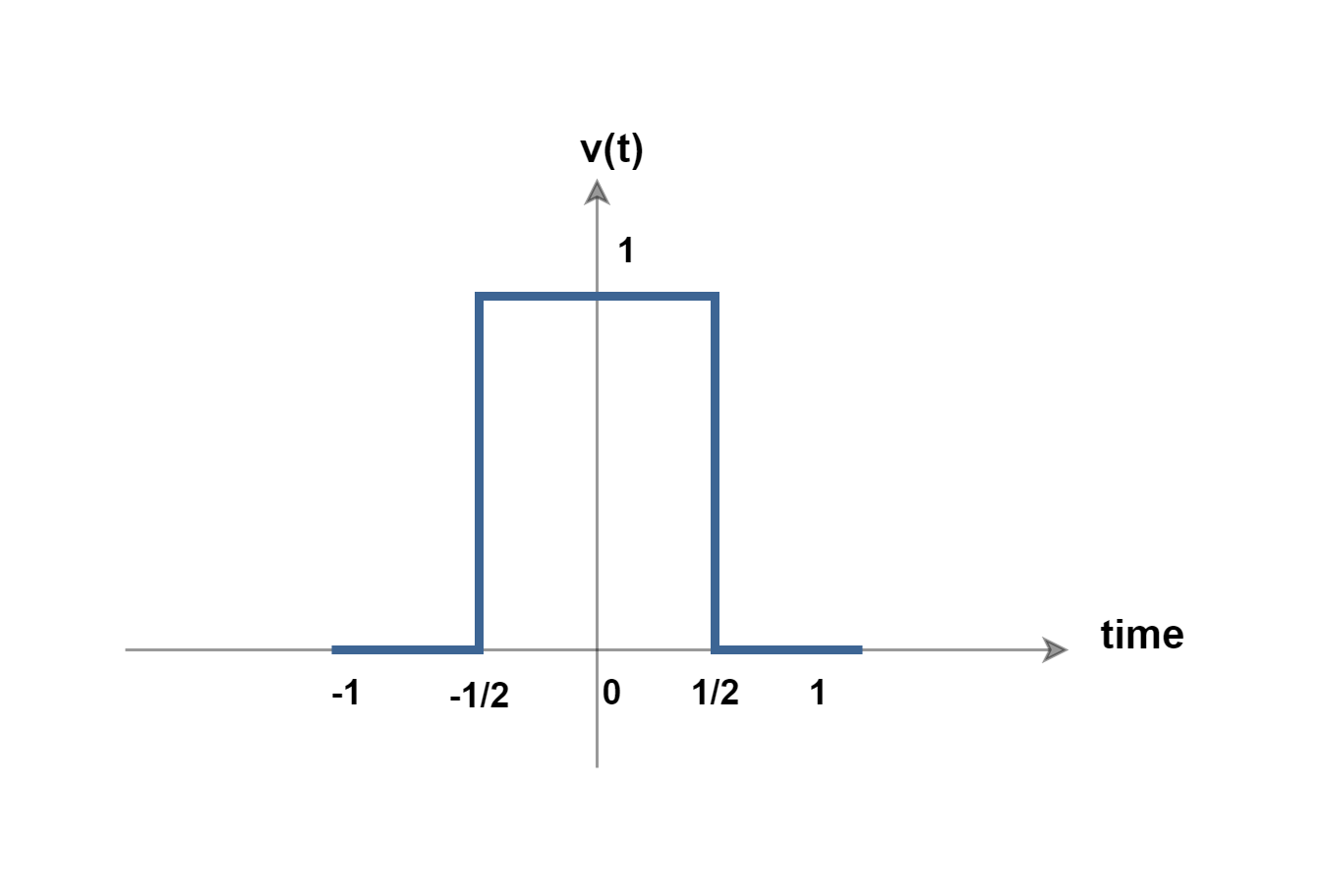
This function can be defined by Equation 7:

If we apply the Fourier transform to this function, we can write Equation 8-1 to calculate the transform:

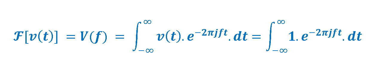
Finally, the result is obtained as Equation 8-2:

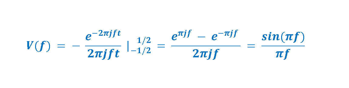
Where the result is simplified by using Euler’s identity to replace two complex exponentials.

The graph of this V(f) is shown in Figure 5:

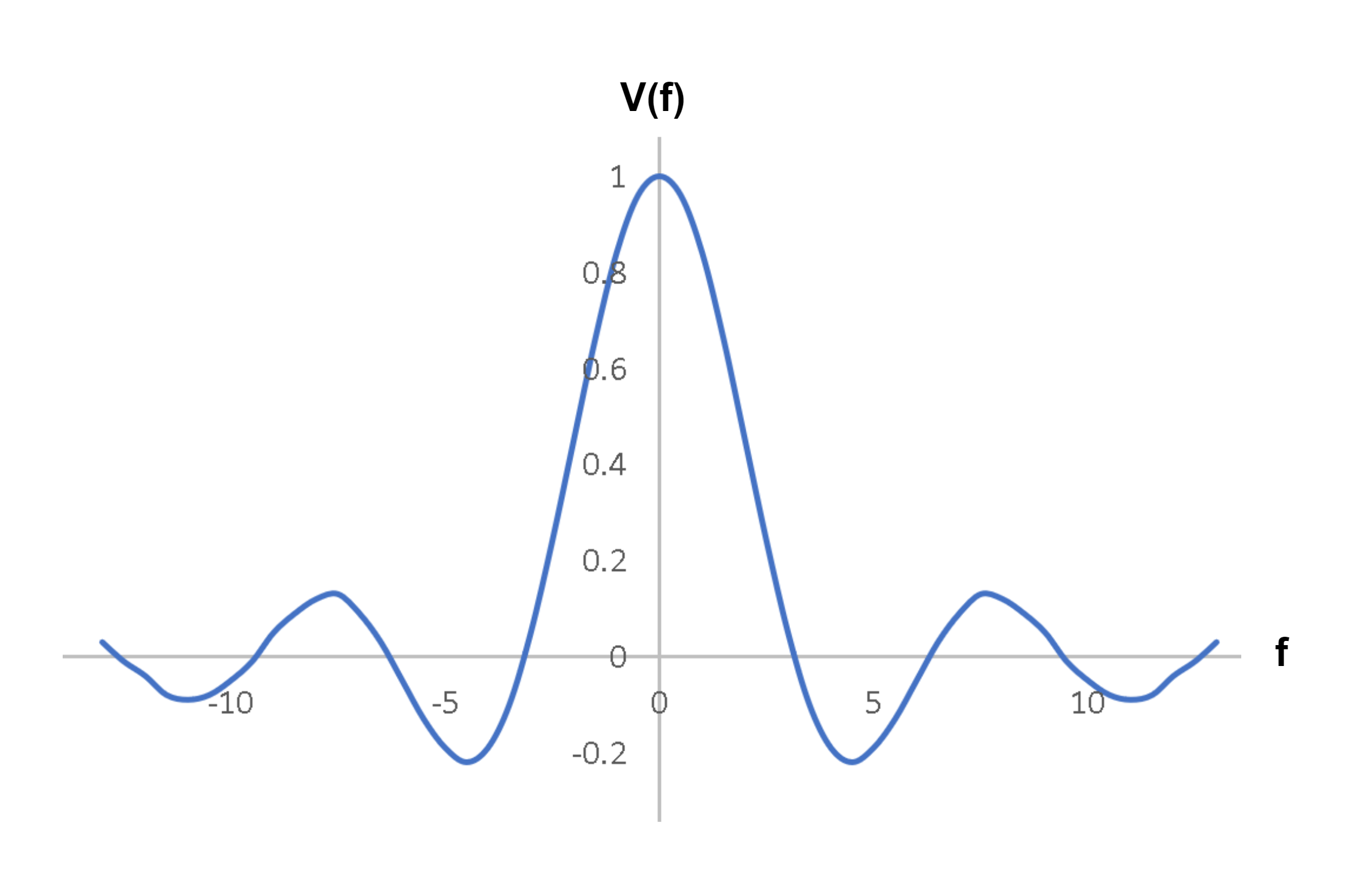
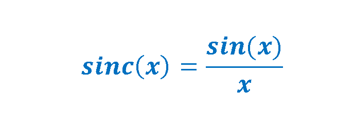
This curve represents one of the classic Fourier transforms with the special function which is called Sinc. Generally, this function is defined as in Equation 9-1 and 9-2:

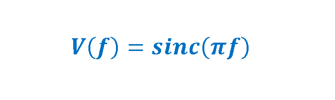
Therefore, we can write our resultant in terms of the Sinc function as in Equation 10:

One property is clear V(f) seems to exist for all values of frequency. The spectrum mathematically consists of positive and negative frequencies, although, the negative frequency range does not practically provide any additional information about the original time domain signal.

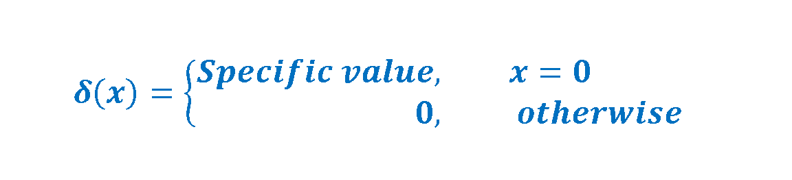
One of the important examples of the Fourier analysis is the unit impulse function which is also called the Dirac delta distribution. In mathematics, the Dirac delta distribution (δ) is a generalized function over the real numbers, whose amplitude value is zero everywhere except at zero. Equation 11 gives the definition of this function:

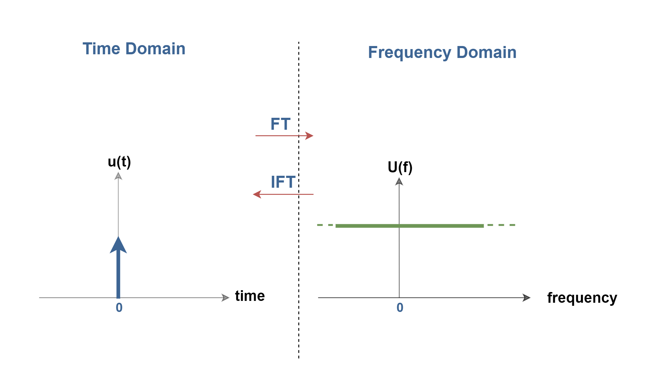
We observed that the spectrum of a single square-wave pulse is a sin(x)/x function. It can be imagined that if the pulse width T₀ is allowed to become narrower to tend towards zero in the time domain, all zero-crossing points of the sin(x)/x function in the frequency domain will tend towards infinity. In the time domain, this provides an infinitely short pulse, a so-called Dirac impulse, the Fourier Transform of which is a straight horizontal line; i.e. the energy of the signal is distributed uniformly from zero frequency to infinity. Figure 6-1 shows u(t) as a unit impulse signal (with an arrow in the graphical representation) and its spectrum as U(f).

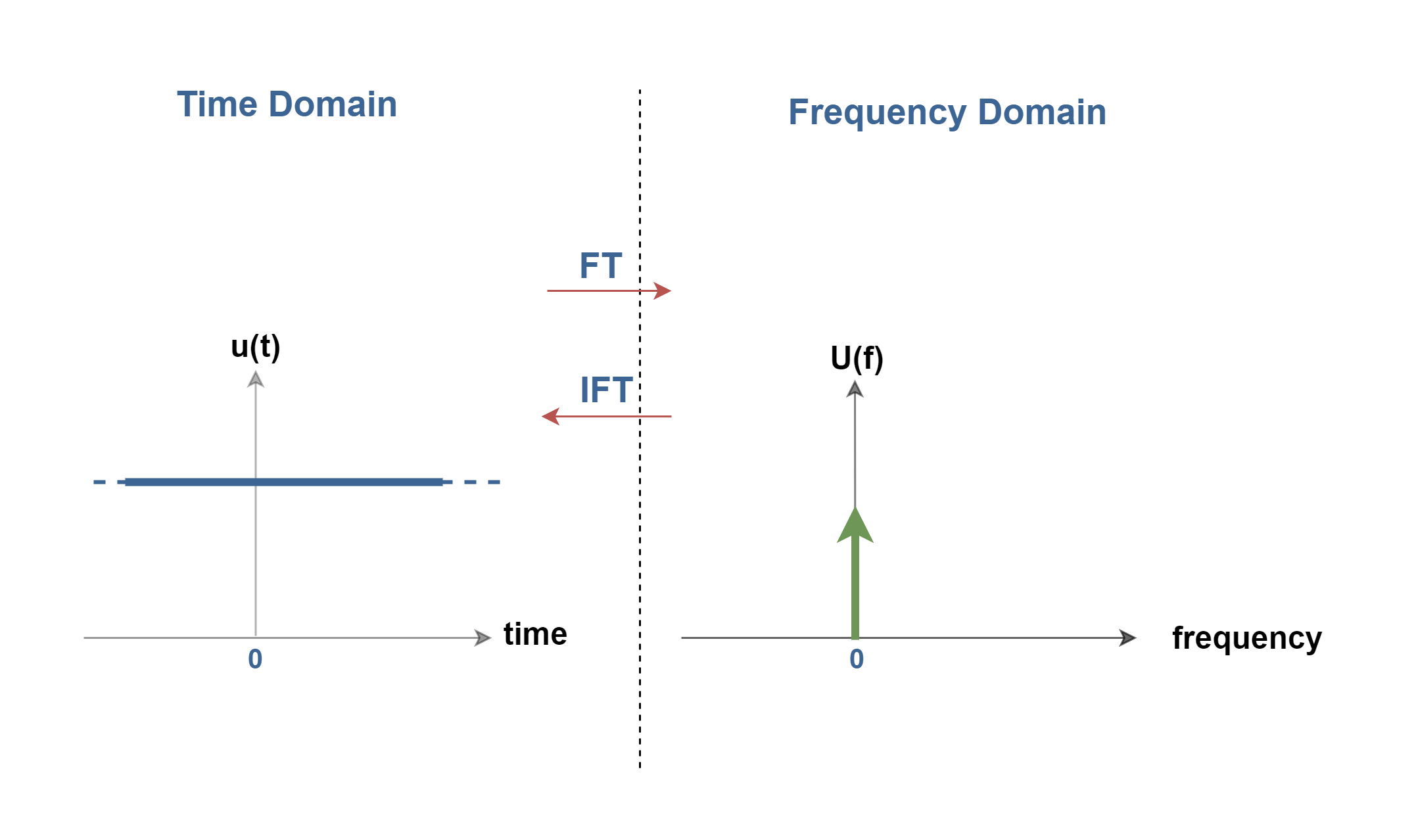
Conversely, a single Dirac needle at f=0 in the frequency domain corresponds to a direct voltage (DC) in the time domain.

Relations Between the Transform and the Inverse Transform

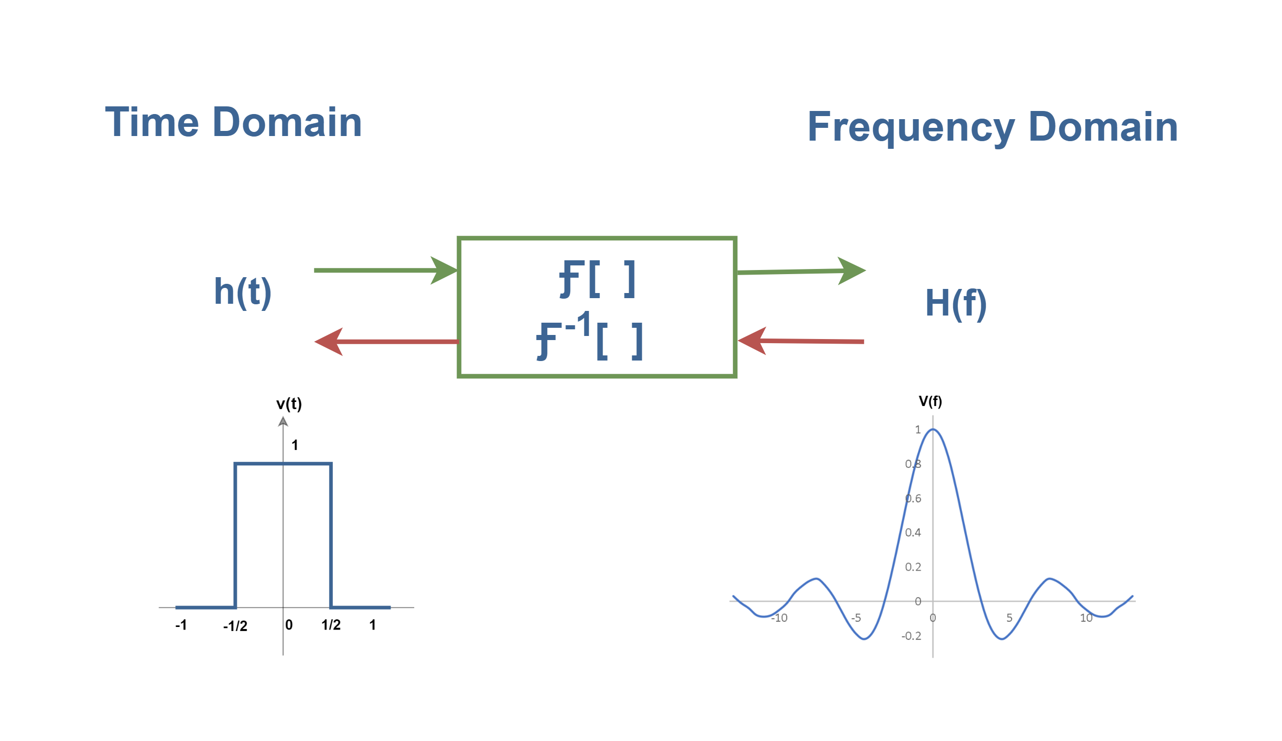
Transforms can be equally well specified either analytically (i.e. by a formula) or graphically. Therefore, we may think of the Fourier transform as a black box or a system whose inputs and outputs are graphs. The central idea of this view is that transforms are functions indeed. The difference is that for a transform, the inputs and outputs are not numbers, but other functions.

The transform pair is completely defined by displaying the respective graphs of the time-domain function as the input and the frequency-domain function as the output (or vice versa) by giving their formulas.

For example, we could view the relationship between the square pulse and its Fourier-transformed function (a sinc function) as shown in Figure 7:

Conclusion

The Fourier Transform calculates the variation of the real components and the variation of the imaginary components versus frequency from the time-domain signal.

The time and frequency parameters of pulsed signals are related in a mutual fashion. This is called the reciprocal spreading principle of signals between time and frequency domains in the Fourier transform concept. It simply means that a wide pulse has a narrow spectrum, whereas a narrow pulse has a wide spectrum. Also, as a spectrum gets wider, its amplitude gets smaller. Using such reciprocal-spreading relationships permits easy time-to-frequency and frequency-to-time conversions.

Now, we can conclude that the Fourier series, i.e. the analysis of the harmonics, is nothing else than a special case of a Fourier Transform where the Fourier Transform is simply applied to a periodic signal and the integral can then be replaced by a summation formula. The information over one period is sufficient for the integration.

Summary

• A transform allows us to see a signal from a different dimension or point of view.
• The Fourier series and its further refinements, such as the Fourier transform, are a form of math that takes a function of one variable (such as time) to another (such as frequency). Hence this type of process is classified as a transform.
• For the nonperiodic signalthe spectral band contains spectral amplitude values not only at certain points but at all points.
• Apart from the fact that a phasor rotates, it has exactly the same properties as any other vector.
• The Fourier transform of a function is a complex-valued function representing the complex sinusoids that contain the original function.
• This transform provides information about the real part, i.e. the cosine component, and the imaginary part, i.e. the sine component, at any point in the spectrum.

Please follow and like us: